Introduction
In today’s rapidly evolving industrial landscape, the seamless collaboration between humans and robots is essential for safety and efficiency. We present a multi-robot shared perception approach that enables mobile robots to anticipate and understand human actions. By combining spatial understanding based on the relation between the human and the surrounding objects and developing a temporal link between frames with decentralized communication among multiple robots, our system ensures that robots can accurately predict human behavior and respond appropriately in dynamic environments.
Following are the main contributions of this paper:
- Development of a spatial understanding block that utilizes graph neural networks, understanding the relations between the subject (human) and the nearby objects using simple attributes.
- A temporal understanding block that aggregates the spatial understanding of other robots in a decentralized manner and predicts and forecasts the action of the human in the scene.
- Enhancing the distributed shared perception pipeline by incorporating a swarm intelligence-inspired consensus mechanism that ensures that the decisions of all the robots converge.
Explore this page to dive deeper into the workings of this model. For an overview, see the video below.
System Architecture
Our multi-robot shared perception system comprises three main components: Spatial Understanding, Temporal Understanding, and Consensus Mechanism. These components work together to process visual data, understand the spatial relationships within the environment, capture the temporal dynamics of human behavior, and ensure that all robots agree on the prediction of human actions.
Spatial Understanding
To accurately infer human actions, our system first processes visual data to understand the spatial relationships within the environment. Using YOLOv8 for object detection, we identify key objects and the human subject in each frame. These detections are then transformed into graph structures where nodes represent objects and edges encode their spatial relationships based on Euclidean distances.
Components:
- Object Detection: Identifying relevant objects using YOLOv8.
- Feature Extraction: Utilizing ResNet50 to generate feature vectors for objects and humans.
- Graph Structures: Creating star-shaped graphs centered around the human subject.
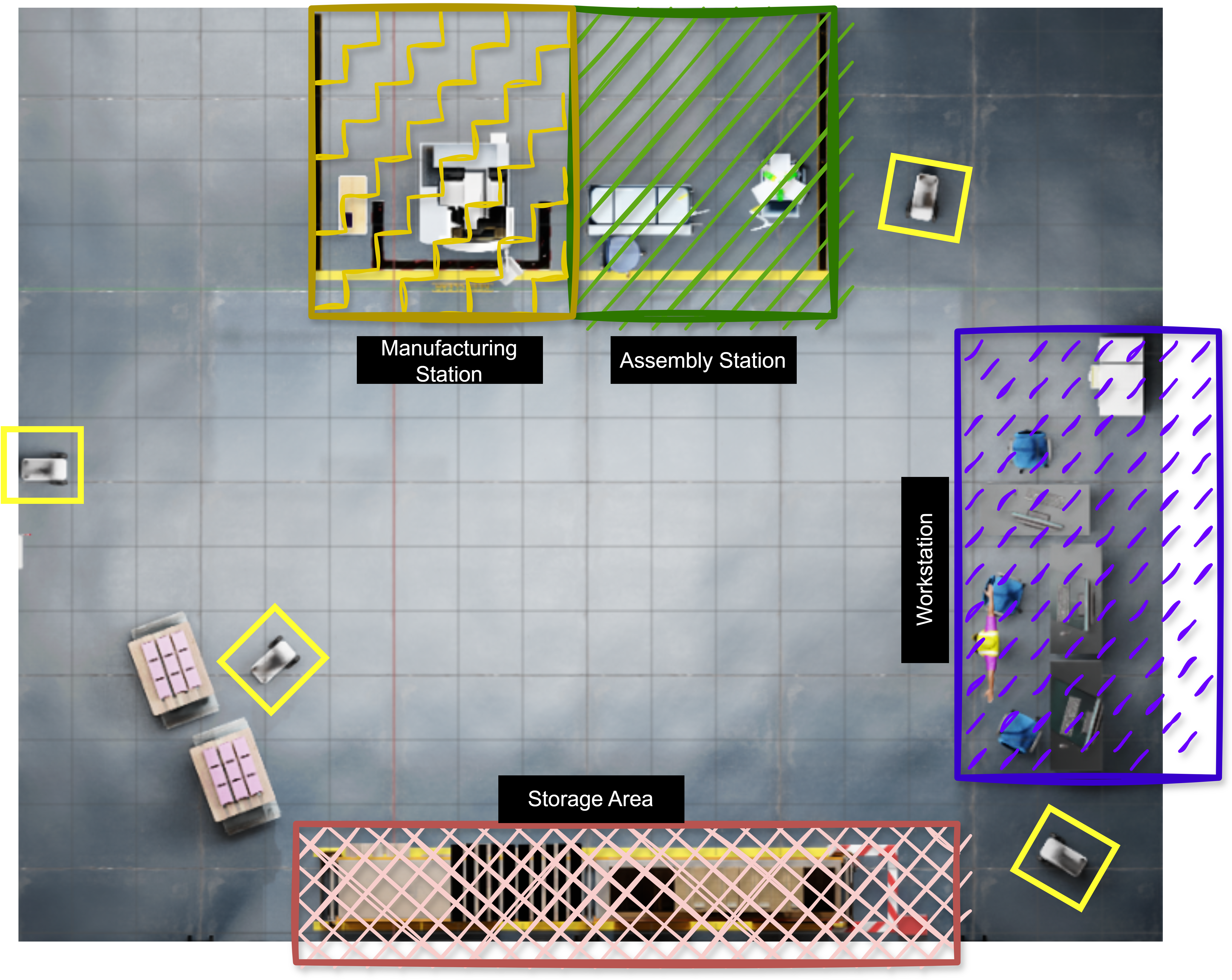
Objects of Interest
| Serial No. | Category | Objects |
|---|---|---|
| 1 | Storage Area | Crates, Boxes, Pallets |
| 2 | Workstation | Desks, Chairs, Storage Drawers, Computers |
| 3 | Assembly Station | Workbench, Chair |
| 4 | Manufacturing Station | CNC Machine, Table |
Graph Neural Networks (GNNs)
Enhancing Spatial Understanding with GNNs
Our framework employs Graph Convolutional Networks (GCNs) to process the graph-structured data, capturing the spatial relationships between the human and surrounding objects. By using a lightweight 2-layer GCN, we ensure efficient onboard processing suitable for real-time applications on mobile robots.
We denote a graph as \( G = (V, E) \), where \( V \) is the set of nodes and \( E \) is the set of edges. The adjacency matrix \( A \in \mathbb{R}^{N \times N} \) for a graph with \( N \) nodes is defined such that \( A_{ij} = 1 \) if there is an edge between node \( i \) and node \( j \), and \( A_{ij} = 0 \) otherwise. The degree matrix \( D \in \mathbb{R}^{N \times N} \) is a diagonal matrix where each diagonal element \( D_{ii} \) represents the degree of node \( i \), i.e., the number of edges connected to node \( i \).
To account for self-loops, we modify the adjacency and degree matrices. The modified adjacency matrix becomes \( A' = A + I \), where \( I \) is the identity matrix. The entries of the modified adjacency matrix \( A' \) are defined as:
\[ A'_{ij} = \begin{cases} 1 & \text{if } i = j, \\ 1 & \text{if there is an edge between } i \text{ and } j, \\ 0 & \text{otherwise}. \end{cases} \]
The modified degree matrix is updated accordingly as \( D_{ii} = \sum_{j} A'_{ij} \). We represent the node features at layer \( l \) with the matrix \( H^{(l)} \in \mathbb{R}^{N \times F^{(l)}} \), where \( F^{(l)} \) is the number of features per node at that layer. The input feature matrix \( H^{(0)} \) has dimensions \( N \times F^{(0)} \), and the output feature matrix \( H^{(L)} \) has dimensions \( N \times F^{(L)} \), where \( L \) is the total number of layers. The weight matrix at layer \( l \) is denoted as \( W^{(l)} \in \mathbb{R}^{F^{(l)} \times F^{(l+1)}} \).
The operation of a GCN layer is represented as:
\[ H^{(l+1)} = \sigma \left( \tilde{D}^{-1/2} \tilde{A} \tilde{D}^{-1/2} H^{(l)} W^{(l)} \right), \]
where \( \tilde{A} = A + I \) is the adjacency matrix with added self-loops, \( \tilde{D} \) is the corresponding degree matrix, and \( \sigma \) is a non-linear activation function—we selected ReLU for our implementation.
The message passing for each node can be expressed as:
\[ h_i^{(l+1)} = \sigma\left( \sum_{j \in \mathcal{N}(i)} \frac{1}{\sqrt{\tilde{D}{ii} \tilde{D}{jj}}} h_j^{(l)} W^{(l)} \right), \]
where \( \mathcal{N}(i) \) denotes the set of neighboring nodes of node \( i \), including itself due to the self-loops.
Temporal Understanding
To capture the temporal dynamics of human behavior, we integrate Gated Recurrent Units (GRUs) into our framework. We utilize two types of GRUs:
- Ego-GRU: Processes information from the individual robot.
- Collective-GRU: Aggregates information from multiple robots to enhance prediction accuracy.
Implementing these two GRUs allows us to gain insights into the multi-robot system. We can evaluate how a single robot performs in understanding the spatial scene and processing temporal information. Additionally, we can assess the improvement in prediction accuracy when a robot incorporates information from other robots, as well as how much it contributes to the overall prediction accuracy of the system.
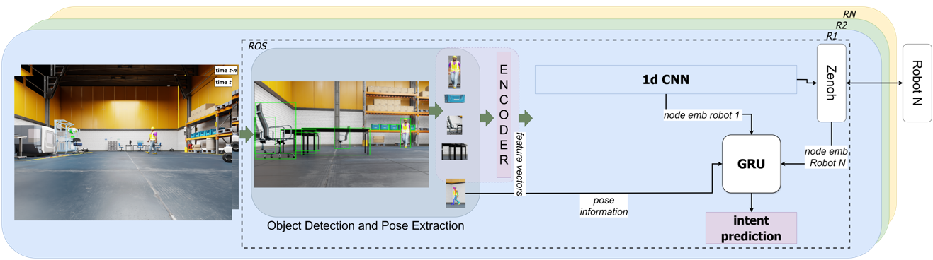
The input vectors for the ego-GRU and collective-GRU are illustrated in the figure below. For the ego-GRU, we concatenate the output of the final layer of the GNN—which is a 1D vector of length 128—with the flattened output of the YOLOv8 keypoints detector (a 1D vector of length 34). In the case of the collective-GRU, an additional information block is concatenated that aggregates the node embeddings (outputs of GNNs from other robots). We employ a simple aggregation strategy by averaging all the node embeddings. It is important to note that this input format is adaptable and scalable to a large number of robots, as all inputs are aggregated to a fixed-sized vector.
Consensus Mechanism
To ensure that all robots agree on the prediction of human actions, we implement a consensus algorithm inspired by swarm intelligence. This mechanism aggregates individual predictions weighted by visibility and confidence levels, allowing the system to converge on a single, robust decision.
Features:
- Weighted Voting: Balances input based on each robot’s visibility and prediction confidence.
- Robustness: Enhances system reliability even with varying numbers of robots.
- Scalability: Maintains decision accuracy as the number of robots increases.
Algorithm Overview:
- 1. Collect visibility, prediction, and confidence from all robots.
- 2. Normalize visibility and confidence scores.
- 3. Weight each prediction based on normalized values.
- 4. Select the prediction with the highest weighted vote as the consensus.
Algorithm: Multi-robot Consensus
Input: Visibility \(v_i\), Prediction \(\hat{p}_i\), Confidence \(c_i\) from all robots.
Output: Consensus prediction \(\hat{p}^*\), Number of participating robots \(n\).
- Initialize action library: \(\mathcal{A} = \{0, 1, 2, 3\}\).
- For each robot \(i\) from 1 to \(n\):
- Collect visibilities \(\mathcal{V} \gets \{v_i\}\), predictions \(\mathcal{P} \gets \{\hat{p}_i\}\), and confidences \(\mathcal{C} \gets \{c_i\}\).
- Calculate number of robots \(n \gets |\mathcal{V}|\).
- If \(n > 1\), normalize visibility and confidence scores:
- \(\tilde{\mathcal{V}} \gets \left\{ \dfrac{v_j}{\sum_k v_k} \ \middle| \ v_j \in \mathcal{V} \right\}\)
- \(\tilde{\mathcal{C}} \gets \left\{ \dfrac{c_j}{\sum_k c_k} \ \middle| \ c_j \in \mathcal{C} \right\}\)
- If \(n = 1\), use unnormalized values for visibility and confidence.
- Initialize weights for each action: \(w(a) \gets 0\), for all \(a \in \mathcal{A}\).
- For each robot \(j\), update the weights for the predicted action \(\hat{p}_j\):
- \(w(\hat{p}_j) \gets w(\hat{p}_j) + w_v \tilde{v}_j + w_c \tilde{c}_j\)
- Select the consensus prediction \(\hat{p}^*\) as the action with the highest weight: \(\hat{p}^* \gets \arg\max_{a \in \mathcal{A}} w(a)\).
Return: \(\hat{p}^*\), \(n\).
Validation of the Consensus Mechanism
To properly validate our consensus mechanism, we needed to verify the relationship between the key parameters it uses: visibility ratio, prediction confidence, and actual prediction accuracy. We conducted a correlation analysis to determine if these parameters are effective foundations for our weighted voting system.
Using Spearman's rank correlation coefficient (ρ) to account for potentially non-linear relationships in our dataset, we observed:
- Visibility ratio and prediction accuracy: A moderate positive correlation (ρ = 0.53, p < .04), indicating that as robots' visibility increased, their prediction performance generally improved.
- Prediction confidence and accuracy: A strong positive correlation (ρ = 0.71, p < .04), suggesting that our internal confidence metric reliably indicates prediction quality across varying scenarios.
The moderate correlation value for visibility can be explained by an interesting trade-off: robots positioned farther from the scene achieve higher visibility ratios by capturing a more holistic view, but simultaneously sacrifice the detailed perspective needed to discriminate between closely positioned potential destinations. This becomes particularly significant when the human's intended destinations are close to one another.
This analysis validates our weighted consensus approach. By assigning greater influence to robots with higher visibility ratios and more confident predictions, the system prioritizes more reliable sources of information. The combination of these two parameters forms a strong foundation for a reliable and robust consensus mechanism, allowing the multi-robot system to weigh predictions based on both environmental perception quality and internal model certainty.
Experimental Setup
Given the dynamic nature of our experimental setup, we evaluated our approach using a comprehensive strategy that assesses the system's ability to infer human actions under varying conditions. We designed three distinct scenarios within the simulation environment, each with an increasing level of difficulty, to test the robustness and adaptability of our system in action inference.
Scenario 1: Ideal Conditions
In the first scenario, there are no obstacles present in the environment, and the robots remain stationary. This setting allows the human worker to move in a straight path toward the intended station.
Scenario 2: Static Obstacles Introduced
In the second scenario, we introduce static obstacles into the environment while keeping the robots stationary. The presence of obstacles forces the human to navigate around them, resulting in less predictable trajectories.
Scenario 3: Dynamic Environment with Moving Robots
The third scenario is the most complex and dynamic. In addition to static obstacles, the robots are also moving within the environment. This creates a highly dynamic setting where both the human and the robots are in motion, and the scene changes continuously.
Furthermore, to increase the complexity of the action inference task, we placed two of the stations in close proximity to each other. This arrangement tests the system's ability to distinguish between similar actions when potential destinations are very close together, making the prediction task even more challenging.
Evaluation Videos
Following videos that demonstrate the three evaluation scenarios in action:
Scenario 1
Scenario 2
Scenario 3
Layout
The layout of the environmet:
Results and Discussion
Our multi-layered, multi-robot perception strategy enhanced the robustness of predictions, especially in dynamic environments. The system processed images at 10 Hz, with performance evaluated across three increasingly difficult scenarios. As complexity increased, the system’s accuracy decreased, as shown in the tables below.
Performance Across Scenarios
We observed that the collective-GRU outperformed the ego-GRU in all cases, especially in more complex scenarios. The consensus mechanism also played a key role in stabilizing overall performance by weighting predictions based on confidence and visibility.
Table 1: Average Accuracy of the Collective-GRU Across Scenarios
| Scenario | GNN (%) | Ego % | Collective % | Consensus (%) | ||
|---|---|---|---|---|---|---|
| t | [1, n] | t | [1, n] | |||
| Scenario 1 | 71.21 | 84.2 | 80.5 | 92.80 | 90.30 | 90.3 |
| Scenario 2 | 73.40 | 82.45 | 79.82 | 91.83 | 91.02 | 89.33 |
| Scenario 3 | 70.73 | 77.7 | 73.5 | 88.87 | 88.1 | 88.5 |
Table 2: Breakdown of the Multi-Robot Perception System
| Robot | GNN (%) | Ego % | Collective % | Consensus (%) | ||
|---|---|---|---|---|---|---|
| t | [1, n] | t | [1, n] | |||
| Robot 1 | 69.2 | 76.1 | 72.3 | 86.3 | 86.1 | 88.5 |
| Robot 2 | 72.90 | 79.2 | 75.1 | 91.8 | 90.5 | 88.5 |
| Robot 3 | 70.1 | 77.8 | 73.10 | 88.5 | 87.8 | 88.5 |
| Overall | 70.73 | 77.7 | 73.5 | 88.87 | 88.1 | 88.5 |
Impact of Robot Count, Time Horizon and Frame Count
Increasing the number of robots improved the accuracy of action inference, as shown in Figure 1. However, the improvement was less pronounced when adding a fourth robot, likely due to lower-quality contributions from one robot. This suggests diminishing returns beyond a certain number of robots, though larger swarms tend to be more fault-tolerant. Using longer time windows for observation (e.g., 3 seconds) led to inconsistent results due to the dynamic nature of the scene, as shown in Figure 2. A 2-second observation window proved optimal, balancing accuracy and computational efficiency. Utilizing more frames for prediction (10 frames vs. 5 or 3) enhanced accuracy, as shown in Figure 3, highlighting the importance of sufficient temporal data for accurate action inference.
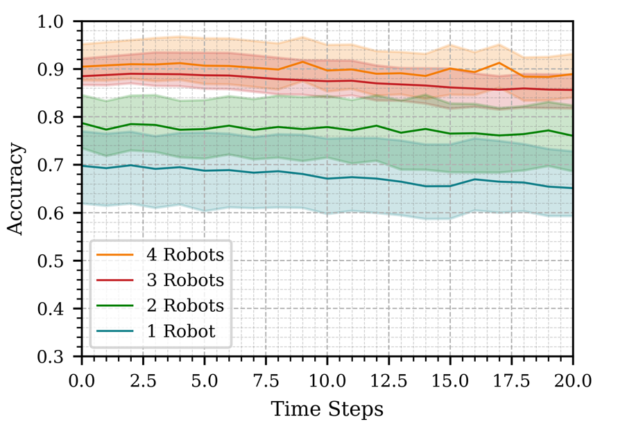
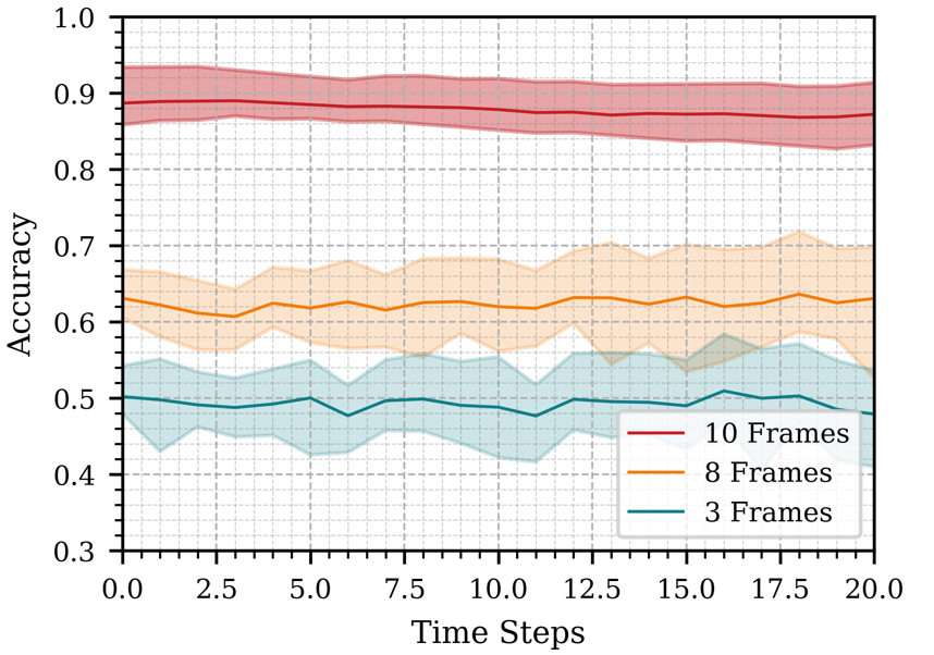
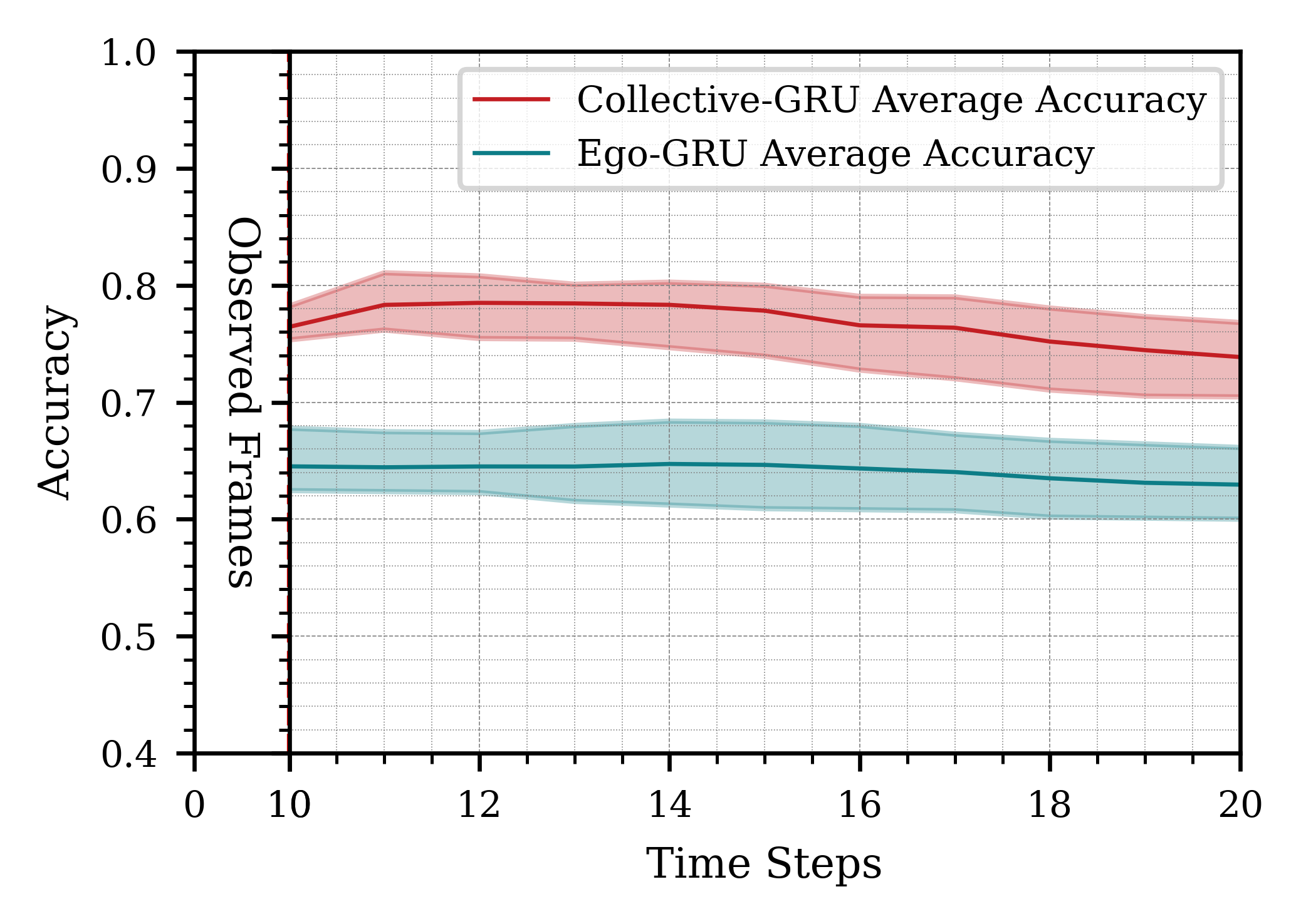
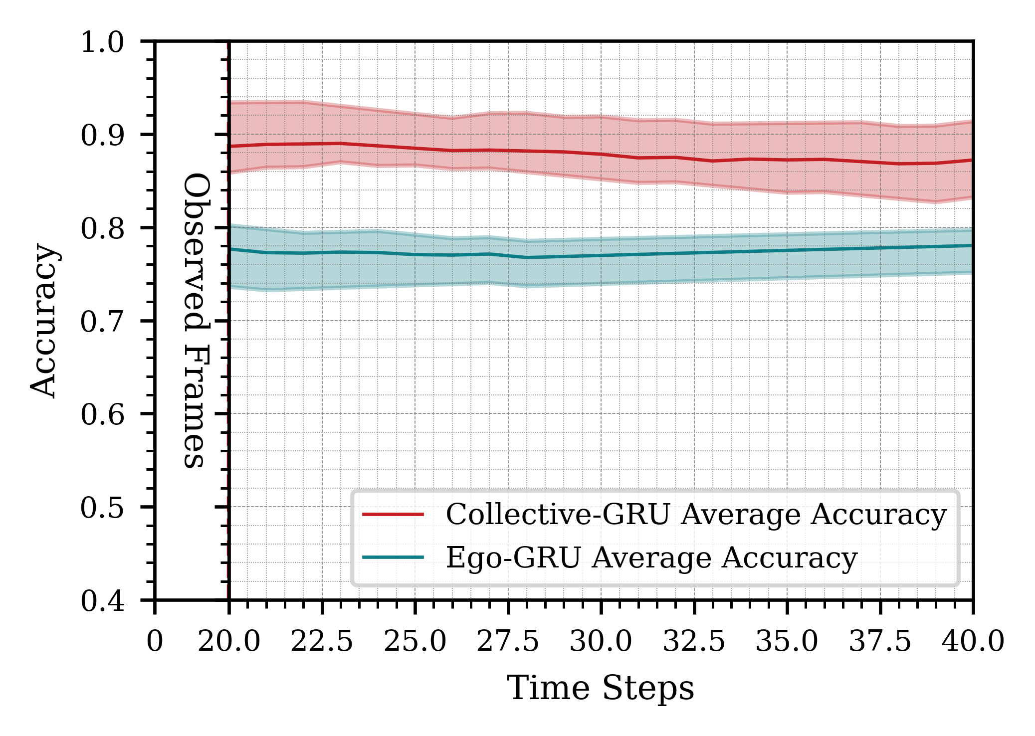
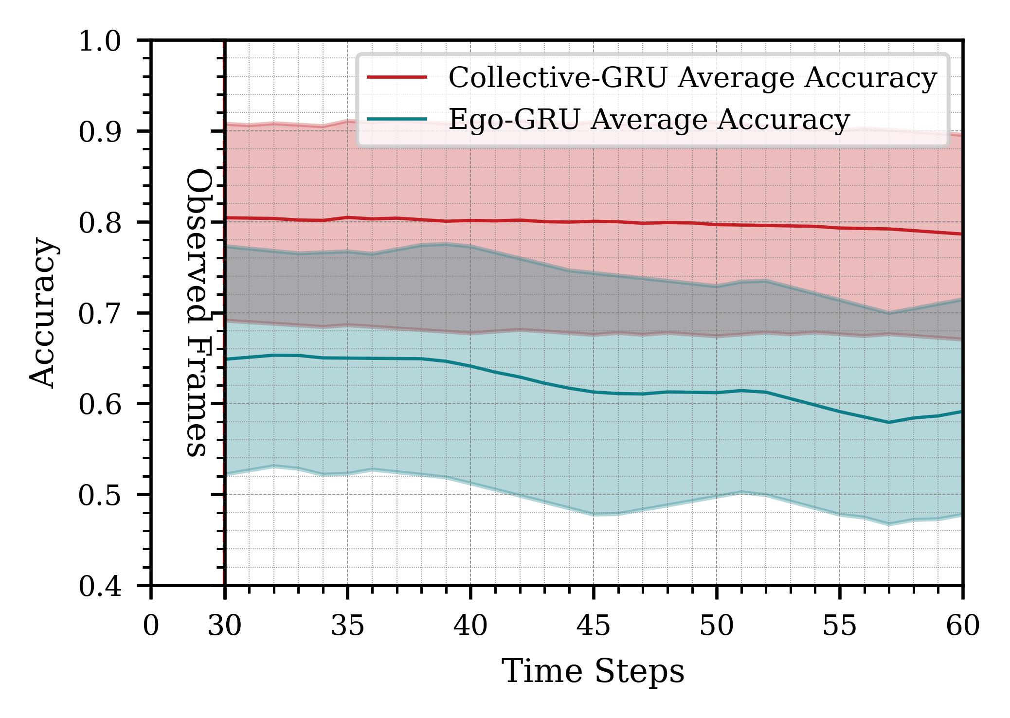
Figure 3: Impact of observing different amounts of information from the past and predicting for a certain time horizon in the future.
Additionally, a noticeable drop in performance was observed for the two stations placed in close proximity to each other.
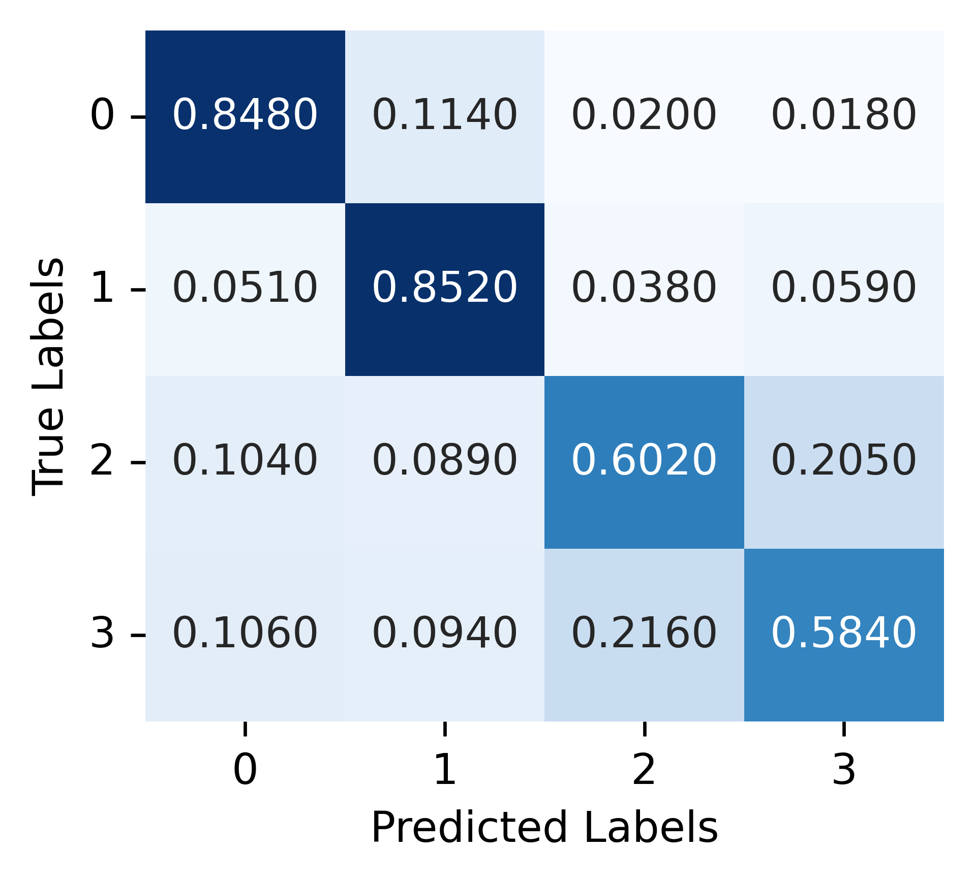
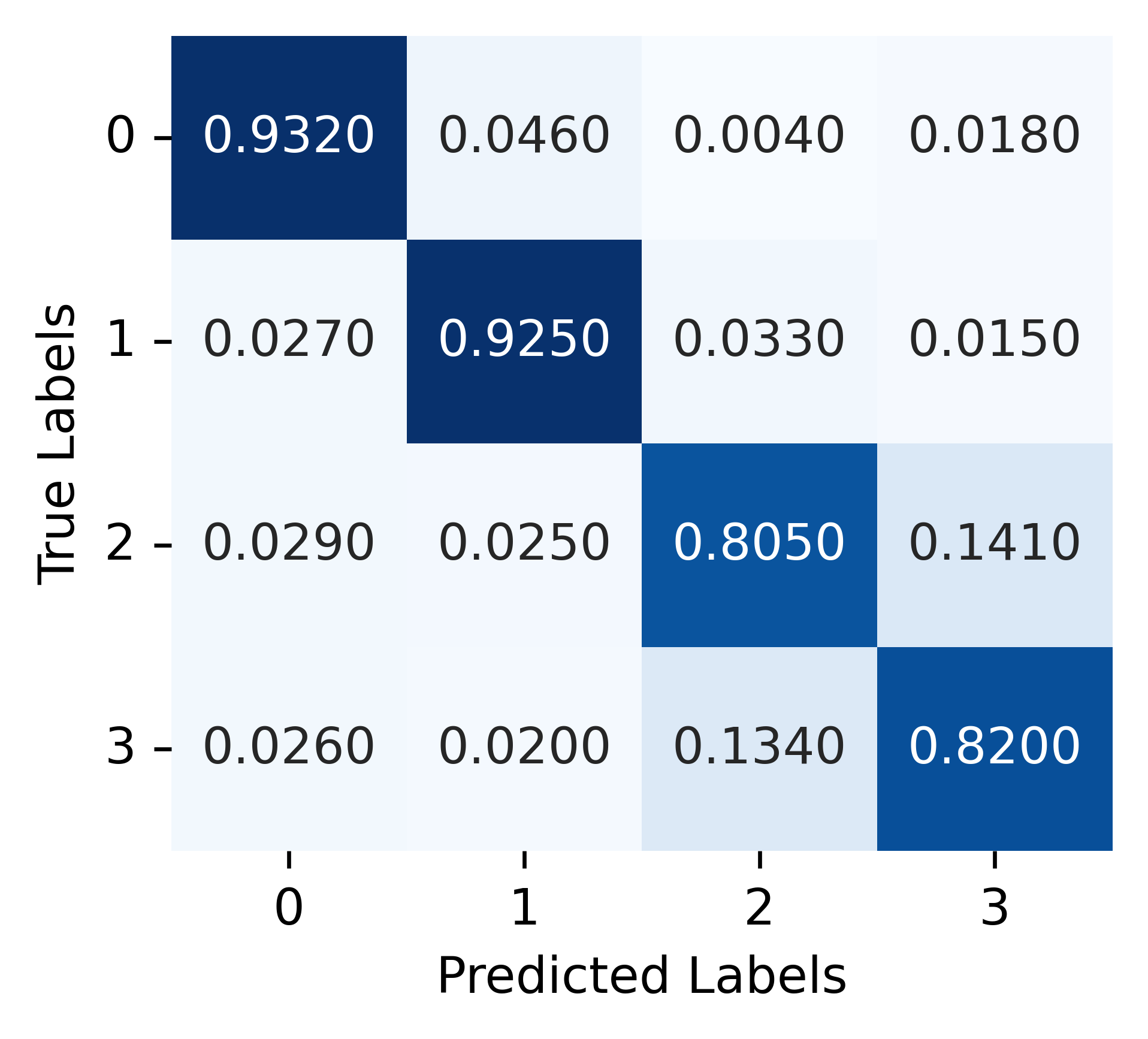
Figure 4: Misclassification on actions between Assembly Station (class 2) and Manufacturing Station (class 3), located close to each other. Left: Ego-GRU, Right: Collective-GRU.
Comparison with Alternative Strategies
We compared our results with two alternative approaches inspired by prior work: a constant velocity model (CVM) and a one-dimensional convolutional neural network (1D-CNN). The CVM is a non-deep learning method that predicts future states based on simple velocity assumptions. The 1D-CNN serves as a baseline to assess whether simpler models suffice without the need for graph neural networks (GNNs). Since our input data is one-dimensional, a 1D-CNN aligns well with it. The results, presented in the table below, are from Scenario 3 of the simulation, using a 2-second temporal window at 10 Hz.
Constant Velocity Model (CVM)
For the CVM, we tracked the human's head using YOLOv8 to obtain keypoints and integrated a Kalman filter for temporal tracking. We used 12 past states to calculate the average velocity and forecast future positions. While the CVM performs well in Scenario 1, where there are no obstacles and the human moves in a straight path, it fails to provide accurate predictions when the human changes direction, remains stationary, or stops.
One-Dimensional Convolutional Neural Network (1D-CNN)
We implemented a simple five-layer 1D-CNN architecture, modifying the input and output to match our application. The node feature of the human served as input. The output was integrated with GRUs, functioning similarly to our spatiotemporal pipeline. Our spatiotemporal approach outperforms the 1D-CNN, demonstrating the effectiveness of integrating spatial and temporal information through GNNs and GRUs.
Performance Comparison of Models
| Serial No. | Model | Avg on Frame $t$ |
|---|---|---|
| 1 | GNN | 70.73% |
| 2 | Ego-GRU | 77.7% |
| 3 | Collective-GRU | 88.87% |
| 4 | CVM | 66.1% |
| 5 | 1D-CNN | 63.31% |
| 6 | Collective-GRU + Consensus | 88.5% |
Sim to Real Gap
Bridging the gap between simulation and real-world deployment involves addressing several challenges. In this section, we analyze how camera sensor noise and communication failures affect our system's performance, and validate our consensus mechanism.
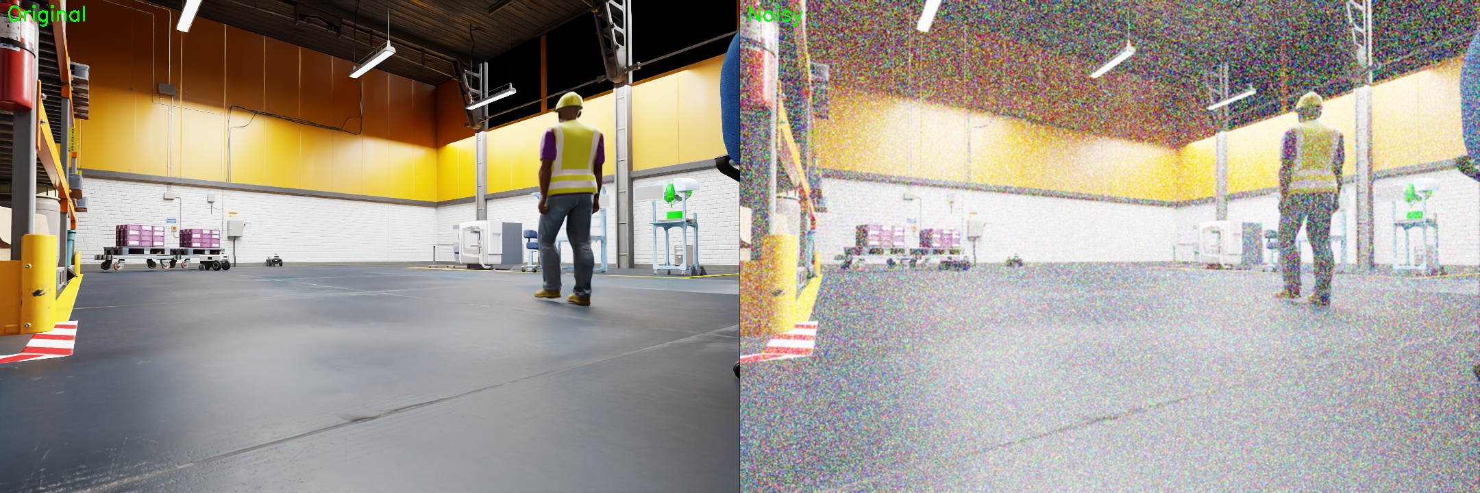
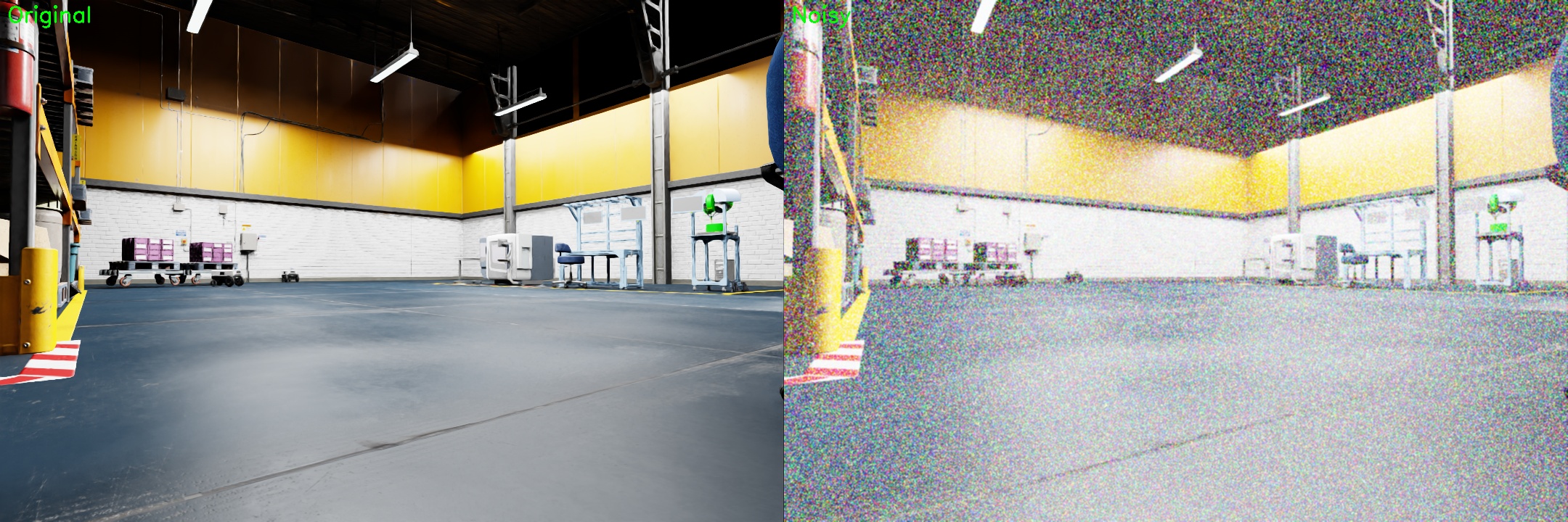
Camera Sensor Noise
The primary sensor for all robots in our system is the camera, and overall performance depends largely on the quality of received images. To systematically analyze the impact of sensor noise, we introduced increasing levels of degradation to the input images on the validation set. The noise injection process involved three stages:
- Blurriness with a kernel size of 3.
- Blurriness (kernel size 3) + white noise with a standard deviation of 0.5.
- Blurriness (kernel size 3) + white noise with a standard deviation of 5.
These experiments were conducted in a 3-robot setup where the robots remained stationary to isolate the effects of sensor noise. The results indicate that performance degrades progressively as noise increases. This degradation begins at the object detection stage (YOLO), leading to lower-confidence predictions, which propagate through the GNN and ultimately affect GRU-based decision-making.
Despite this effect, our multi-robot system demonstrated resilience: as detection failures increased, the system dynamically adjusted by switching to fewer-robot cases. When a robot's camera became unreliable, it relied solely on the predictions of neighboring robots, mitigating the impact of sensor noise.
Performance metrics under different blur and noise conditions
| Metrics | Blur: 0 Noise: 0 |
Blur: 3 Noise: 0.5 |
Blur: 3 Noise: 3 |
Blur: 3 Noise: 5 |
|---|---|---|---|---|
| Failed detections (%) | 28 | 51.4 | 72 | 95.33 |
| Avg Object Detection Conf (%) | 94.8 | 94.7 | 93.9 | 86.1 |
| Avg number of nodes | 8 | 8 | 7.8 | 7.9 |
| Human detection rate (%) | 72 | 71.1 | 65.2 | 59 |
| GNN Accuracy (%) | 85 | 62 | 40.5 | 15.7 |
| Ego-GRU accuracy (%) | 87.2 | 61.56 | 51.1 | 20.1 |
| Ego-GRU conf | 0.84 | 0.85 | 0.76 | 0.77 |
| Consensus Accuracy (%) | 92.1 | 89.2 | 88.2 | 88 |
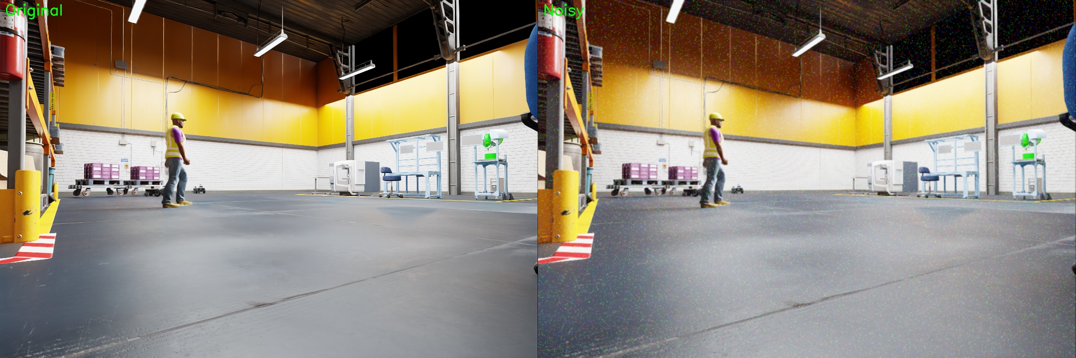
Effects of Blur and Noise on Image Quality
Communication Failures
To evaluate the system's robustness to communication failures, we conducted additional experiments with a static 4-robot scenario, designed to highlight the impact of communication loss.
We compared system performance under two conditions: one with no packet loss, and another with an induced packet loss of approximately 30% according to Bernoulli distribution. The results indicate that the system dynamically transitions between different operational modes — switching between the collective GRU and ego GRU configurations based on the information available from other robots.
Without packet loss, the system primarily operates in the three-robot and four-robot configurations, demonstrating stable performance. However, with induced packet loss of 30%, the system dynamically adjusts based on the number of robots successfully transmitting data. When communication loss prevents certain robots from sharing information, the system automatically falls back to fewer-robot cases, ensuring continued functionality.
Performance comparison with varying packet loss rates
| Robots | ploss: 0 | ploss: 0.3 | ||
|---|---|---|---|---|
| Samples | Acc | Samples | Acc | |
| GNN | 164 | 84.2 | 164 | 84.1 |
| Ego-GRU | 155 | 86.5 | 155 | 86.45 |
| GRU - 2 robots | 0 | - | 55 | 90.3 |
| GRU - 3 robots | 39 | 91.1 | 47 | 94.1 |
| GRU - 4 robots | 97 | 96.2 | 13 | 93.1 |
| Consensus | 97 | 96.2 | 13 | 93.1 |
Dynamic GRU Configuration in Communication Scenarios
The figures below illustrate how our system dynamically adapts to different communication conditions. The top subplot in each figure shows the active GRU configuration, which adjusts based on the number of robots successfully exchanging information. The bottom subplot represents the number of robots actively participating in the multi-robot system.
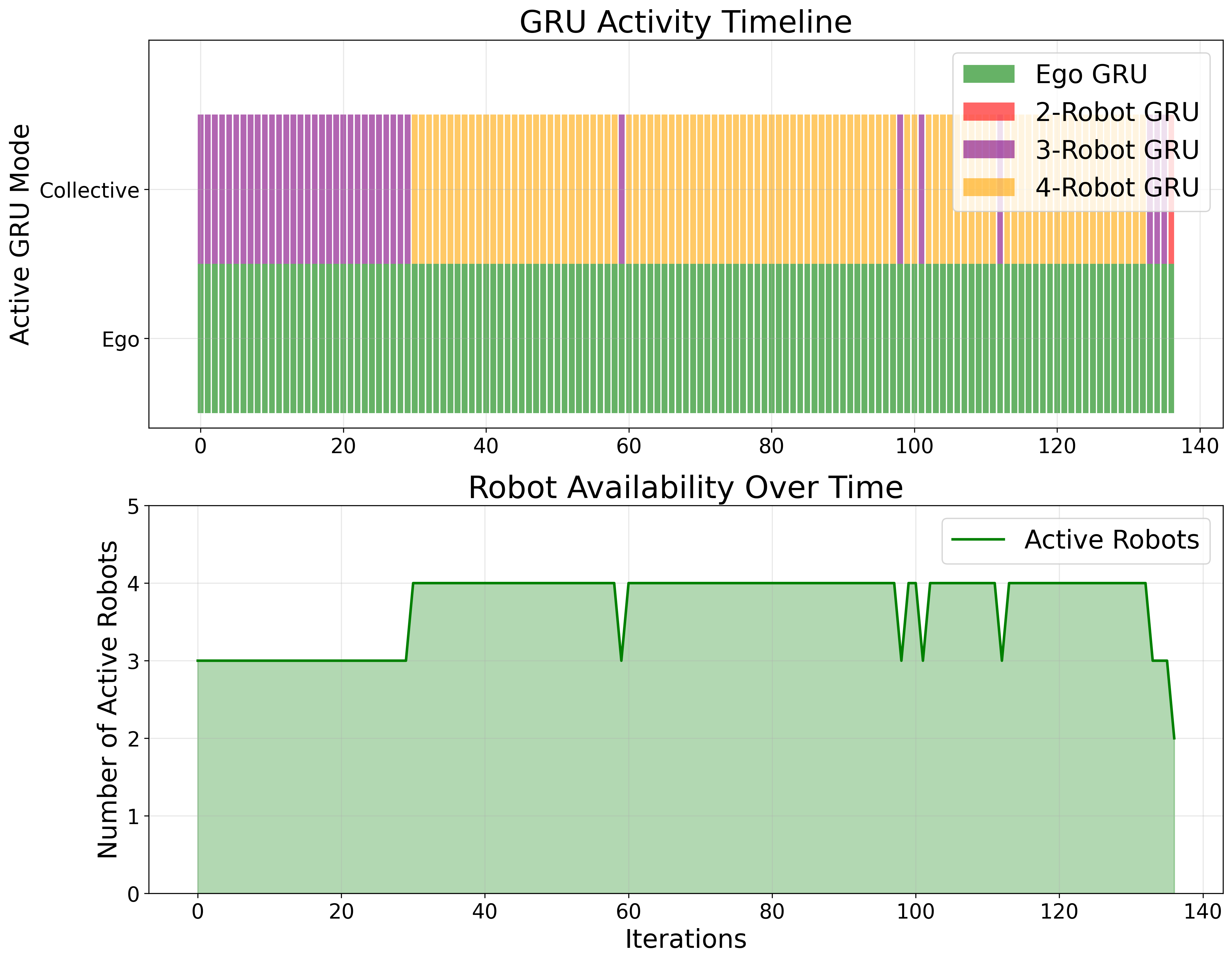
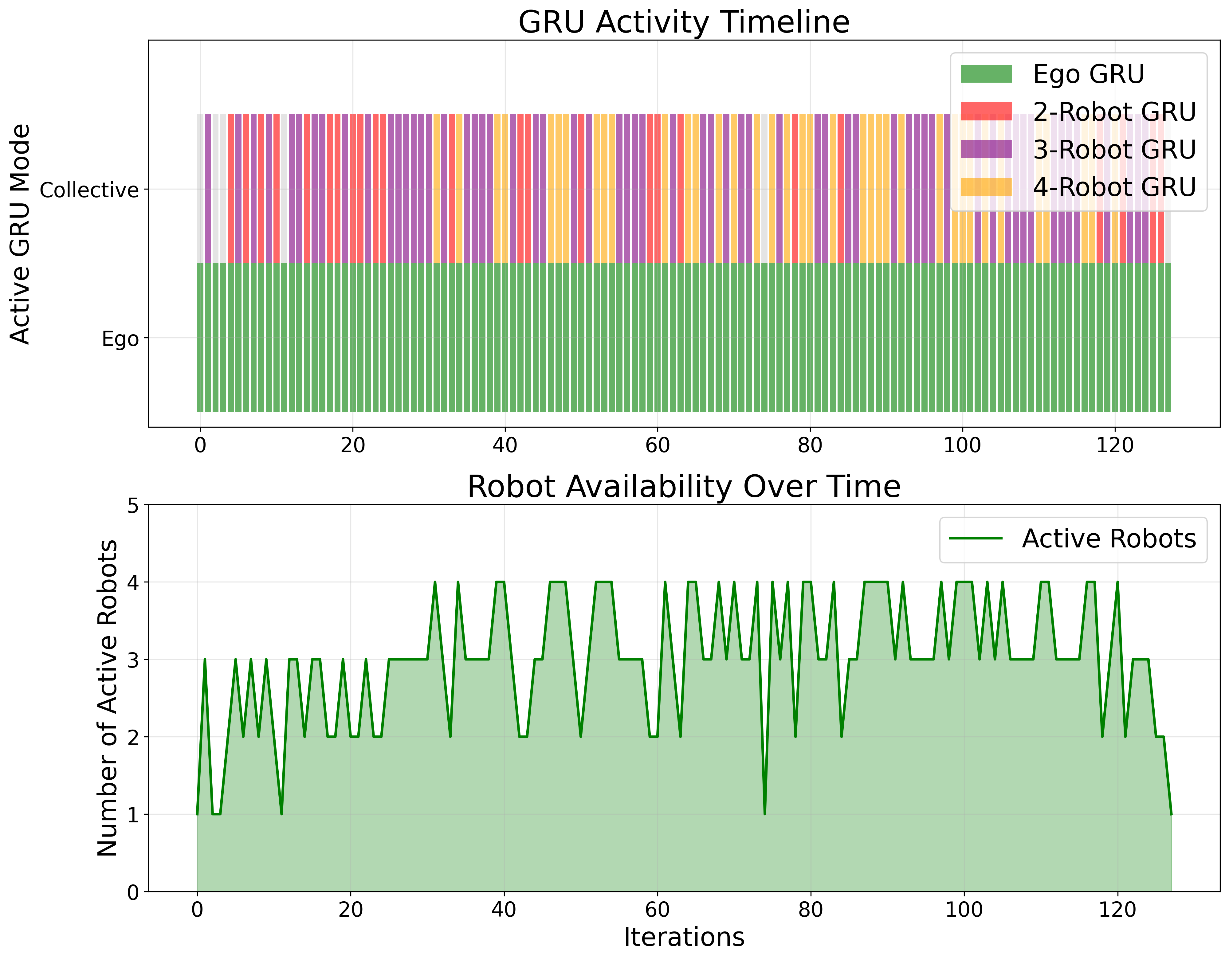
These results demonstrate that the system effectively maintains accuracy while dynamically adjusting to network disruptions. The two-robot GRU, which observes zero samples in the no-packet-loss scenario, becomes active when communication loss occurs. The ego-GRU remains active throughout, as it doesn't rely on information from neighboring robots. This adaptability reinforces the system's robustness to communication failures in real-world scenarios.
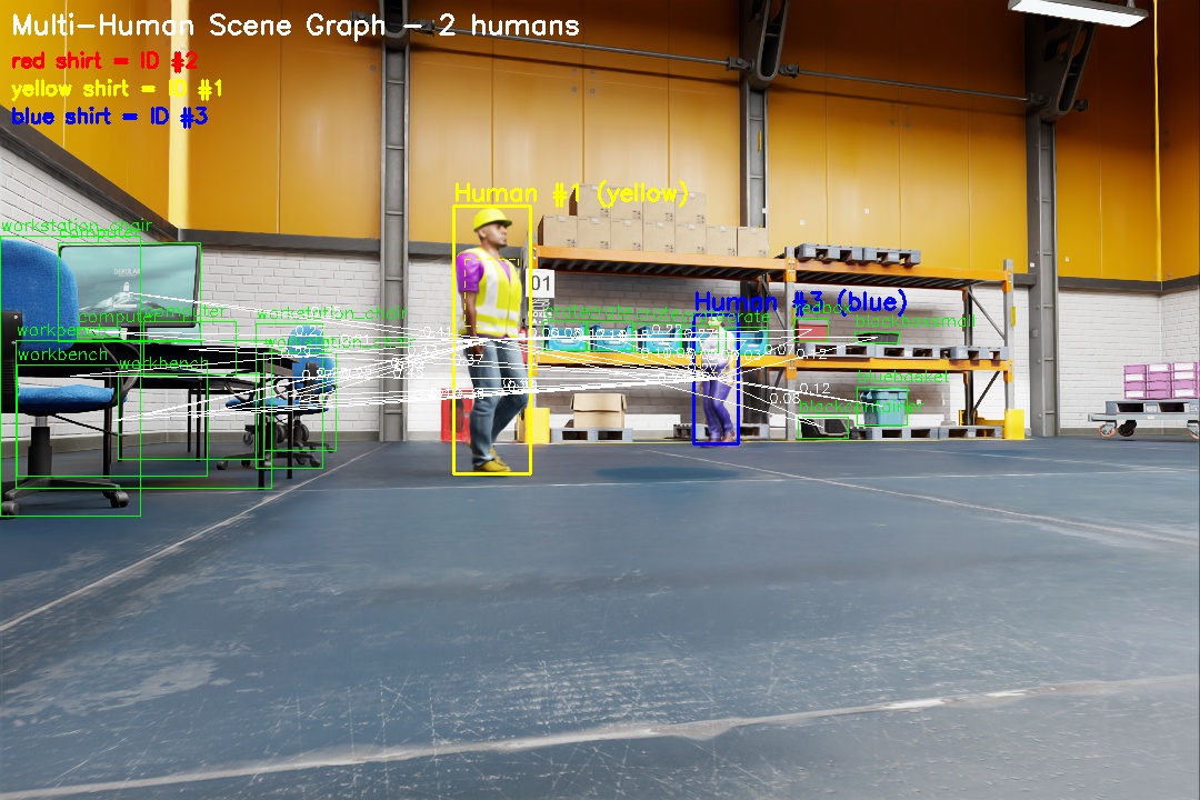
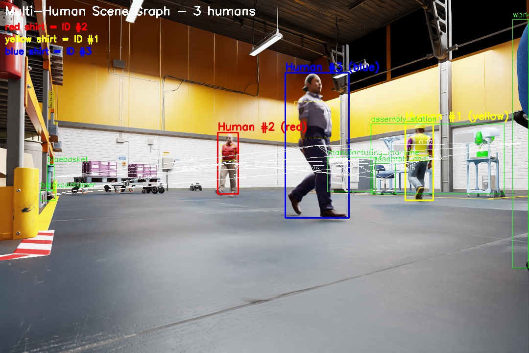
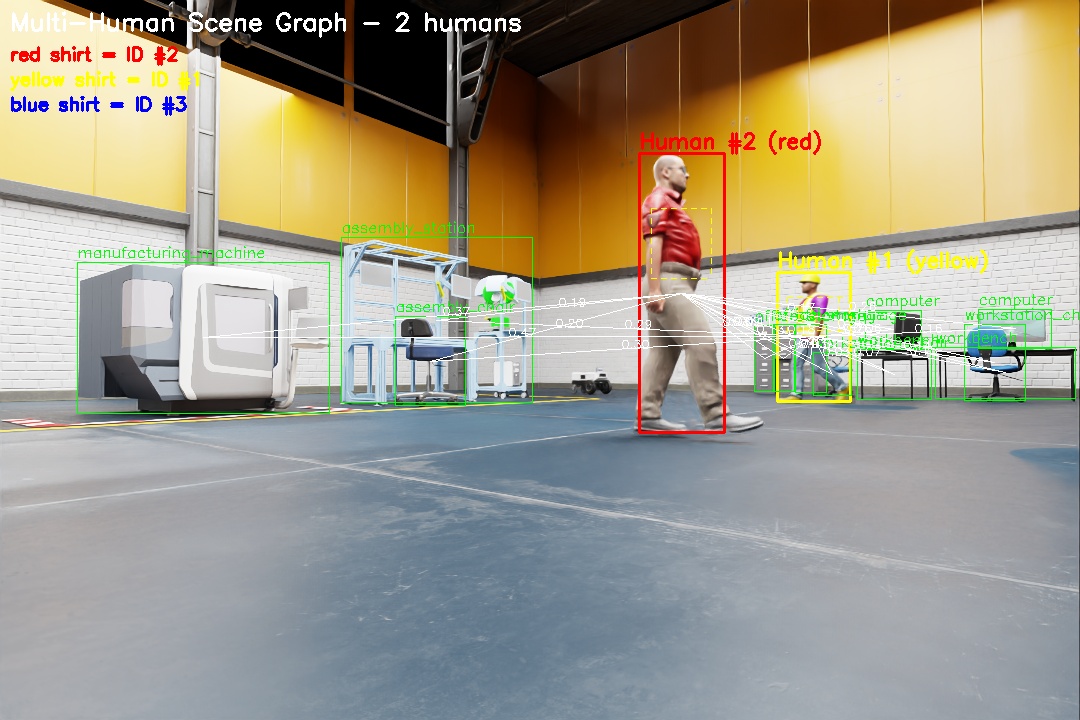
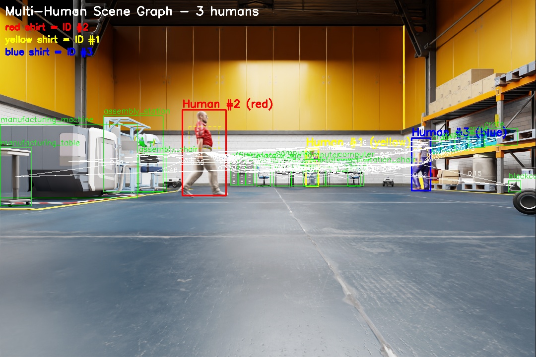
Multi-Human Scenarios
Extending the system's capabilities to handle multiple humans in the scene is a key focus for future work. Predicting intent in multi-human scenarios adds significant complexity, particularly due to the interactions between individuals, which affect the graph structures. Nevertheless, our system can already accommodate multi-human scenarios with the assumption of no relationship between the humans, i.e., treating each as an independent entity with disconnected graphs.
To enable multi-human tracking, we rely on YOLOv8 tracking. However, tracking the same individual across multiple robots introduced a challenge, as each robot perceives the scene from a different perspective. While various identification techniques exist to address this issue, our primary focus is on evaluating the intent prediction pipeline rather than optimizing human tracking. Therefore, we opted for a simpler approach that assigns global IDs based on distinct clothing colors, ensuring that observations from different robots can be correctly associated without requiring complex re-identification methods (for instance, a human in blue clothing was assigned an ID of 3).
The system effectively handles multiple humans by running independent instances of the GNN and GRU for each human. Since the graphs remain disconnected, each human's intent can be predicted separately.
Multi-Human Multi-Robot Intent Prediction Scenario
Performance Results in Multi-Human Scenarios
The table below presents the results for each human as observed by each robot across all deployed models. The general performance trend — improvement from GNN to ego-GRU to collective-GRU — remains consistent. However, we observe that the prediction accuracy for Human 2 and Human 3 is significantly lower than for Human 1.
| Robot | Model | Human 1 (Yellow) | Human 2 (Red) | Human 3 (Blue) |
|---|---|---|---|---|
| Robot 1 | GNN | 70.22 | 65.6 | 63.33 |
| Ego-GRU | 73.21 | 68.8 | 64.3 | |
| Collective-GRU | 73.12 | 68.7 | 64.1 | |
| Consensus | 78.4 | 70.3 | 69.6 | |
| Robot 2 | GNN | 74.6 | 66.12 | 66.4 |
| Ego-GRU | 79.1 | 60.2 | 68.1 | |
| Collective-GRU | 84.4 | 73.4 | 71.9 | |
| Consensus | 79.5 | 72.1 | 69.9 | |
| Robot 3 | GNN | 72.45 | 70.4 | 62.1 |
| Ego-GRU | 78.9 | 71.4 | 63.9 | |
| Collective-GRU | 82.7 | 77.3 | 68.23 | |
| Consensus | 79.1 | 72.3 | 68.1 | |
| Robot 4 | GNN | 70.7 | 66.1 | 71.1 |
| Ego-GRU | 74.07 | 66.4 | 74.2 | |
| Collective-GRU | 74.23 | 69.2 | 74.0 | |
| Consensus | 79.8 | 71.0 | 69.1 |
We attribute this performance drop to the composition of the training dataset, where only a single human instance (depicted as wearing yellow in the figure) was used, maintaining the same appearance throughout training. Since the model creates node embeddings by combining both human appearance and the surrounding scene, it struggles with generalization when faced with previously unseen human appearances.
Despite this performance gap, the system maintains a consistent trend in prediction accuracy across different configurations. We hypothesize that training the model with diverse human appearances would mitigate this challenge and improve generalization. This will be a focus of future work to enhance the system's scalability in real-world multi-human environments.